Deep Neural Nets for Option Pricing

1. Data
2. Split Into Training and Test Datasets
3. Keras Sequential Neural Network
4. Pytorch

See this paper for an early analysis which used neural nets to learn the Black-Scholes model.

1. Data

The data we'll use is

import pandas as pd
import seaborn as sns
import matplotlib.pyplot as plt
data = pd.read_csv("./data_all_strikes.csv")
data.columns

Index(['tradeDate', 'tradeTime', 'strikePrice_ezOct', 'typeInd_ezOct',
       'deliveryDate_ezOct', 'avgTradePrice_ezOct', 'deliveryDate_esOct',
       'avgTradePrice_esOct', 'timeTillExp', 'IV', 'BS', 'Delta', 'Gamma',
       'Vega', 'Theta', 'Rho', 'moneyness'],
      dtype='object')

data.drop(columns=["tradeDate", "tradeTime", "deliveryDate_ezOct", "deliveryDate_esOct"], axis=1, inplace=True)
## , "BS", "Delta", "Gamma", "Vega", "Theta", "Rho"
data

        strikePrice_ezOct typeInd_ezOct  avgTradePrice_ezOct  avgTradePrice_esOct  ...        Vega       Theta        Rho  moneyness
0                    1915          call                38.50          1924.750000  ...  219.781116 -193.814146  84.322011   1.005091
1                    1775           put                29.50          1925.000000  ...  265.304020 -154.899336 -98.211918   1.084507
2                    1300           put                 1.05          1924.737500  ...   17.230719  -29.597195  -2.497067   1.480567
3                    2025          call                12.25          1925.250000  ...  197.562625 -112.587345  50.271795   0.950741
4                    1450           put                 1.75          1924.500000  ...   30.536723  -42.303744  -4.798547   1.327241
...                   ...           ...                  ...                  ...  ...         ...         ...        ...        ...
162514               2040           put                24.50          2093.250000  ...  269.287036 -163.673642 -90.049373   1.026103
162515               2020           put                 8.00          2094.196918  ...  128.158304 -195.454232 -21.050682   1.036731
162516               2050           put                12.75          2094.196918  ...  164.129275 -228.562824 -32.513976   1.021559
162517               2120          call                12.00          2094.196918  ...  177.471988 -178.721561  37.109958   0.987829
162518               2125          call                10.00          2094.196918  ...  168.685183 -165.809959  33.108156   0.985504

[162519 rows x 13 columns]

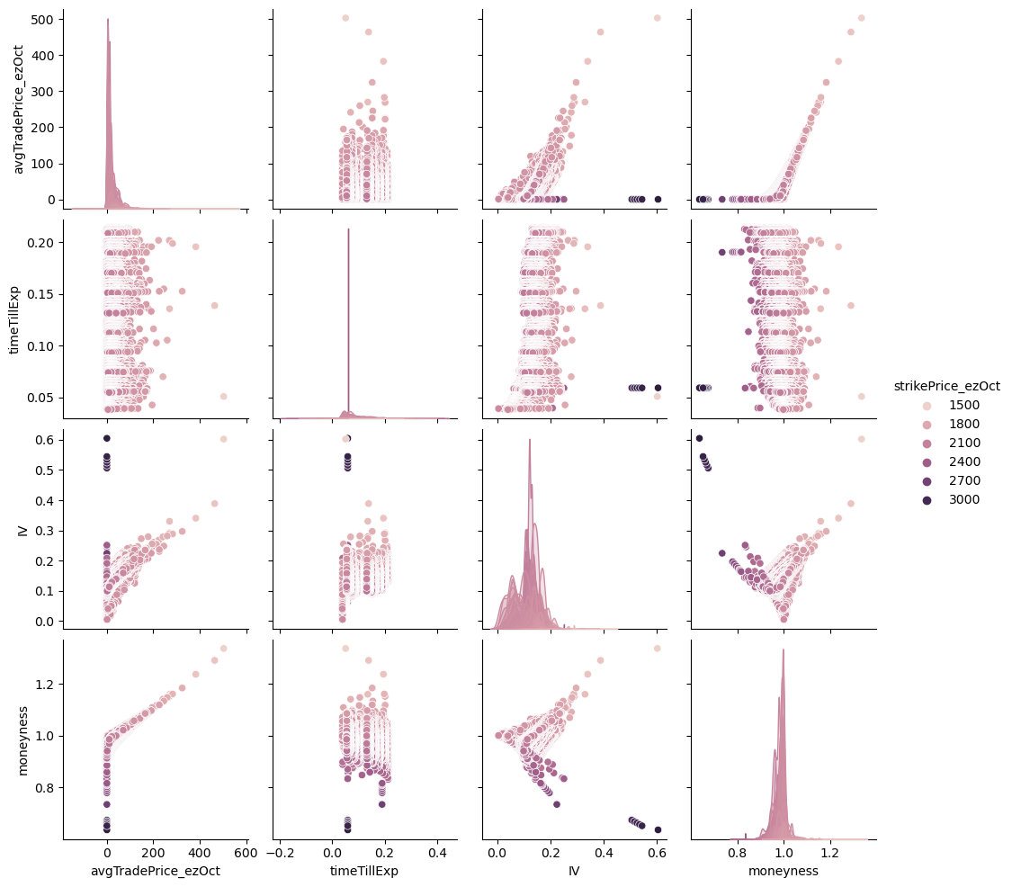
sns.color_palette("viridis", as_cmap=True)
call_plot = sns.pairplot(data[data["typeInd_ezOct"] == "call"][["avgTradePrice_ezOct", "timeTillExp", "IV", "moneyness", "strikePrice_ezOct"]], hue="strikePrice_ezOct")
call_plot.savefig('call_plot.png')

put_plot = sns.pairplot(data[data["typeInd_ezOct"] == "put"][["avgTradePrice_ezOct", "timeTillExp", "IV", "moneyness", "strikePrice_ezOct"]], hue="strikePrice_ezOct")
put_plot.savefig('put_plot.png')

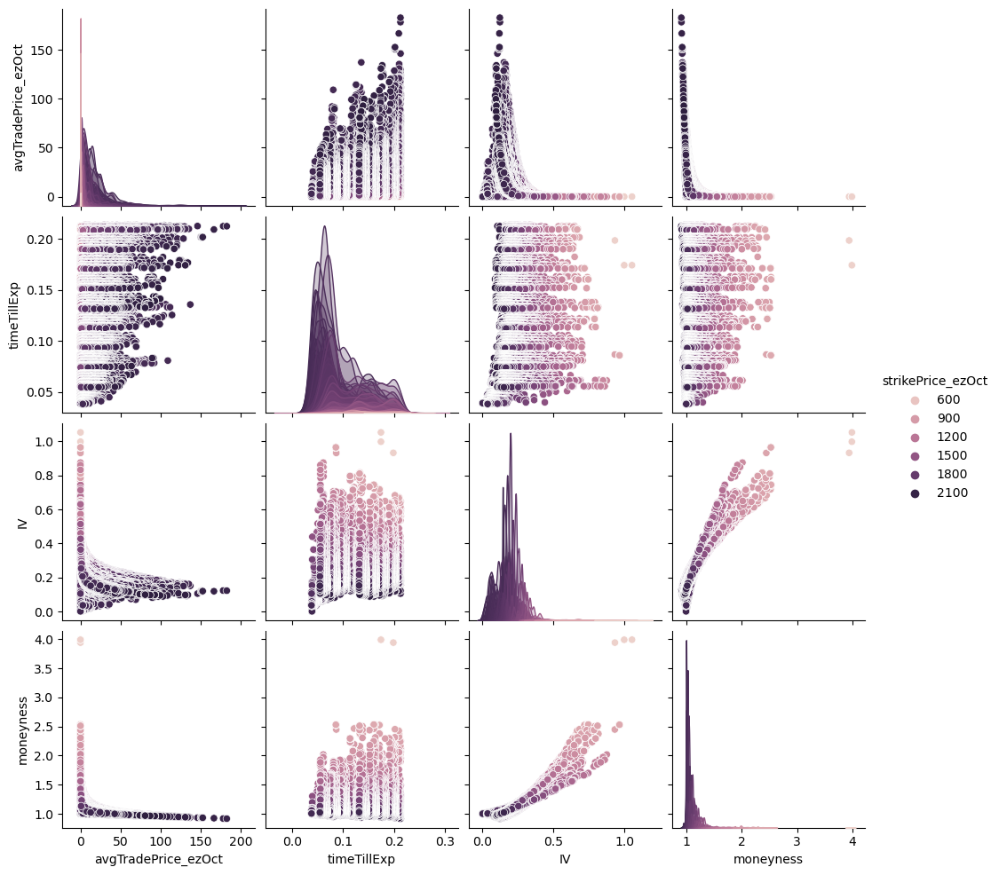
Split into calls and puts.

calls = data[data['typeInd_ezOct'] == 'call']
calls.drop(columns=["typeInd_ezOct"], axis=1, inplace=True)
puts = data[data['typeInd_ezOct'] == 'put']
puts.drop(columns=["typeInd_ezOct"], axis=1, inplace=True)

2. Split Into Training and Test Datasets

from sklearn.model_selection import train_test_split

Create a simple sequential model using Keras.

target_calls = calls['avgTradePrice_ezOct']
features_calls = calls[['avgTradePrice_esOct', 'timeTillExp', 'IV', 'moneyness', 'Delta', 'Gamma', 'Vega', 'Theta', 'Rho']]

features_calls_train, features_calls_test, targets_calls_train, target_calls_test = train_test_split(features_calls, target_calls, test_size=0.33)

3. Keras Sequential Neural Network

# import tensorflow as tf
# from tensorflow import keras
# from tensorflow.keras import layers

4. Pytorch

import torch
device = 'cuda'

fct = torch.tensor(features_calls_train.values, device = device, requires_grad = True)
tct = torch.tensor(targets_calls_train.values, device = device, requires_grad = True)
fcg = torch.tensor(features_calls_test.values, device = device, requires_grad = True)
tcg = torch.tensor(target_calls_test.values, device = device, requires_grad = True)

## code mainly from the Pytorch docs here:  https://pytorch.org/tutorials/beginner/examples_nn/two_layer_net_nn.html


N, D_in, H, D_out = 30, 9, 10, 1  # batch size, dimensions in, hidden layers, dimensions out-----

model = torch.nn.Sequential(
    torch.nn.Linear(D_in, H),
    torch.nn.ReLU(),
    torch.nn.ReLU(),
    torch.nn.Linear(H, D_out),
)

model = model.float()

model.to(device)

loss_fn = torch.nn.MSELoss(reduction='sum')

learning_rate = 1e-8
for t in range(500):
    y_pred = model(fct.float())

    loss = loss_fn(y_pred, tct.float())
    if t % 100 == 99:
        print(t, loss.item())

    model.zero_grad()

    loss.backward()

    with torch.no_grad():
        for param in model.parameters():
            param -= learning_rate * param.grad

calls_test_results = pd.Series(model(fcg.float()).detach().cpu().numpy().reshape(-1))
actual_call_values = pd.Series(target_calls_test.values)

calls_results = pd.concat([calls_test_results, actual_call_values], axis=1)
calls_results.set_axis(["prediction", "actual_price"], axis=1, inplace=True)
calls_results

Deep Neural Nets for Option Pricing

Table of Contents

1. Data

2. Split Into Training and Test Datasets

3. Keras Sequential Neural Network

4. Pytorch