Convexity

1. Bond Convexity
2. Visualizations
3. Calculating Convexity
4. Duration with Convexity Adjustment
5. Duration and Convexity Calculator

1. Bond Convexity

Bond convexity refers to the actual convex (non-linear) relationship between a bond's price and yield. This is stated in relation to the linear duration approximation of the bond price and yield relationship.

Convexity is often used as a general term for the approximation error that exists when using duration to approximate interest rate risk.
The idea is this: duration is a linear (first derivative) approximation. To make the approximation more accurate, we can include a second-derivative adjustment, which is known as the convexity adjustment.
The convexity adjustment is more important as the change in yield increases.
This is most easily understood graphically.

2. Visualizations

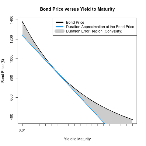
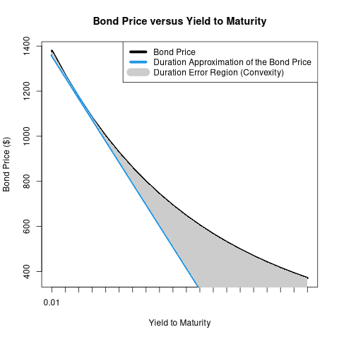
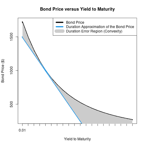
The following series of visualizations allows you to see, for varying yields, a bond's actual price, the price predicted by duration, and the effect of convexity.

Observe that duration always predicts that the bond's price will be lower than it will actually be. Bond owners love convexity!

You can also see the effect of the coupon, YTM, and maturity on the bond's duration and convexity.

A steeper slope means a higher duration (more interest rate risk).
When changing the coupon rate and maturity, note the changing values on the vertical axis to see the slope steepening and flattening.

##Bond Price, Duration, and Convexity
plot_convexity <- function(input_ytm = 0.07, input_coupon = 0.05, input_years = 10){
ytm <- input_ytm
coupon <- input_coupon
years <- input_years

bondValue <- 0
ytmAxis <- seq(0.01, .2, by = .01)
period <- 1

cash_flows <- 0
    for (i in 1:years){
        cash_flows[i] <- 
            (coupon * 1000) }

    cash_flows[length(cash_flows)] <- cash_flows[length(cash_flows)] + 1000 
    pvCashFlows <- cash_flows / (1 + ytm)^(1:years)

## Bond Calculation: includes semiannual case which is not used ----   
     if (period == 1) {
         for (i in seq_along(ytmAxis)){
          bondValue[i] <- (coupon * 1000) * ((1 - 1 / (1 + ytmAxis[i])^(years)) / ytmAxis[i]) + 1000 / (1 + ytmAxis[i])^(years) }
 }    else {
         for (i in seq_along(ytmAxis)){
          bondValue[i] <- (coupon * (1000 / 2)) * ((1 - 1 / (1 + (ytmAxis[i] / 2))^(years * 2)) / (ytmAxis[i] / 2)) + 1000 / (1 + (ytmAxis[i] / 2))^(years * 2)
              }
          }

# find on x-axis where ytm equals the input ytm -----
   index <- seq_along(seq(0.01, .2, by = .01))[round(ytm,2) == round(ytmAxis, 2)]

# Calculate Duration and Modified Duration ----
    Duration <- 1:years %*% (pvCashFlows / bondValue[index])
    modDur <- -1 * Duration / (1 + ytm)
    durLine <- bondValue[index] * (1 + (modDur * (ytmAxis - ytm)))

yAxis <- c("0.01", "", "", "", "0.05", "", "", "", "", "0.10", "", "", "", "", "0.15", "", "", "", "", "0.20")

png(paste0("./img/convexity_", ytm, "_", coupon, "_", years, ".png"))
plot(1:20, bondValue, xaxt = "n", main = "Bond Price versus Yield to Maturity", ylab = "Bond Price ($)", xlab = "Yield to Maturity", type = "n", lwd = 4)
axis(1, at = 1:20, labels = yAxis)
lines(1:20, bondValue, lwd = 4)
lines(1:20, durLine, lwd = 5, col = 4)
legend('topright', c("Bond Price", "Duration Approximation of the Bond Price ", "Duration Error Region (Convexity)"), lty = c(1,1,1,1), col=c(1,4, "grey80"), lwd = c(5,5, 15))
## attempting to shade region between the two lines [not working] ----
polygon(c(1:20, rev(1:20)), c(bondValue, rev(durLine)), col = "grey80", border = NA)
dev.off()
}

plot_convexity(0.07, 0.05, 10)

convexity_0.07_0.05_10.png

plot_convexity(0.03, 0.05, 10)

convexity_0.03_0.05_10.png

plot_convexity(0.05, 0.05, 20)

convexity_0.05_0.05_20.png

3. Calculating Convexity

To approximate the change in the bond's price given a particular change in yield, we add the convexity adjustment to our original duration calculation. Convexity (C) is defined as:

\(C = \frac{1}{P}\frac{\partial^2 P}{\partial y^2}\)
where \(P\) is the bond's price, and \(y\) its yield-to-maturity.

Taking the second derivative of the bond's price with respect to yield affords:

\(\frac{\partial^2 P}{\partial y^2} = \sum_{t=1}^{T} t(t+1)\frac{C_t}{(1+y)^{t+2}}\)
where \(t\) is each period (coupon payment), numbered from \(1\) to \(T\), and \(C_t\) is the payment amount in that period.

4. Duration with Convexity Adjustment

And so the approximation of the change in the bond's price for a given change in yield (\(\Delta y\)), including both duration and convexity, is:

\(\Delta P \approx -D^*P\Delta y + \frac{1}{2}CP(\Delta y)^2\)
where \(D^*\) is the bond's Modified Duration.

On the next slide is an interactive duration and convexity calculator.

import numpy as np

class bond:
    def __init__(self, coupon, years, ytm):
        self.coupon = coupon
        self.years = years
        self.ytm = ytm

    def payments(self):
        self.coupon_payment = (self.coupon * 1000) / 2
        self.periods = np.linspace(1, self.years * 2, self.years * 2)
        self.payments = np.repeat(self.coupon_payment, len(self.periods))
        self.payments[len(self.periods) - 1] = self.payments[len(self.periods) - 1] + 1000
        return self.payments

    def value(self):
        # self.payments()
        self.value = np.inner(self.payments, (self.payments * 1 / (1 + (self.ytm / 2))**self.periods))
        return self.value

    def duration(self):
        # self.payments()
        # self.value()
        numerator_duration = np.inner(self.periods, (self.payments * (1 / (1 + (self.ytm / 2))**self.periods)))
        duration_in_periods = numerator_duration / self.value
        self.macaulay_duration = duration_in_periods / 2
        self.modified_duration_in_years = self.macaulay_duration / (1 + self.ytm / 2)
        return self.modified_duration_in_years

    def convexity(self):
        # self.payments()
        # self.value()
        # self.duration()
        second_derivative = np.inner((self.periods * (self.periods + 1)), ((self.payments * (1 / (1 + self.ytm / 2)**(self.periods + 2)))))
        self.convexity = second_derivative / self.value
        ## annualize semiannual convexity
        self.convexity = self.convexity / (2**2)
        return self.convexity

None

5. Duration and Convexity Calculator

years <- 10
ytm <- 0.1
change_ytm <- 0.01
coupon <- 0.05

## calculate payments ----
coupon.pmt <- (coupon * 1000) / 2
periods <- seq_along(seq(from = 0.5, to = years, by = 0.5))
payments <- rep(coupon.pmt, max(periods))
payments[max(periods)] <- payments[max(periods)] + 1000

## bond value ----
bv <- payments %*% (1 / (1 + (ytm / 2))^periods)

## duration ----
numerator.duration <- periods %*% (payments * (1 / (1 + (ytm / 2))^periods))
duration.in.periods <- numerator.duration / bv
macaulay.duration <- duration.in.periods / 2
## modified.duration.in.periods <- duration.in.periods / (1 + ytm)
## modified.duration.in.years <- modified.duration.in.periods / 2
modified.duration.in.years <- macaulay.duration / (1 + ytm / 2)

## convexity ----
second.derivative <- (periods * (periods + 1)) %*% ((payments * (1 / (1 + ytm / 2)^(periods + 2))))

convexity <- second.derivative / bv

## annualize semiannual convexity
convexity <- convexity / (2^2)

## approximate change in price
price.change.by.duration <- -modified.duration.in.years * bv * change_ytm
price.change.by.duration.convexity <- price.change.by.duration + 0.5 * convexity * bv * (change_ytm)^2

## approximate percent change
percent.change.by.duration <- -modified.duration.in.years * change_ytm
percent.change.by.duration.convexity <- percent.change.by.duration + 0.5 * convexity * (change_ytm)^2
predicted.bv <- bv + price.change.by.duration.convexity 


new.bond.value <- payments %*% (1 / (1 + ((ytm + change_ytm) / 2))^periods)
actual.price.change <- (new.bond.value / bv - 1) * bv
actual.percent.change <- (new.bond.value / bv - 1)

error <- abs(predicted.bv - new.bond.value)

df <- data.frame(c(macaulay.duration, modified.duration.in.years, convexity, percent.change.by.duration * 100, percent.change.by.duration.convexity * 100, actual.percent.change * 100, price.change.by.duration, price.change.by.duration.convexity, actual.price.change, new.bond.value, predicted.bv, error), row.names = c("Macaulay Duration", "Modified Duration", "Convexity", "% Change by Duration", "% Change by Duration and Convexity", "Actual % Change", "Price Change by Duration", "Price Change by Duration and Convexity", "Actual Price Change", "Actual New Price", "Predicted New Price", "Difference: Predicted vs Actual"), stringsAsFactors = "FALSE")

names(df) <- ""

library(xtable)

print(xtable(df), type = "html")


Macaulay Duration	7.49
Modified Duration	7.13
Convexity	64.44
% Change by Duration	-7.13
% Change by Duration and Convexity	-6.81
Actual % Change	-6.82
Price Change by Duration	-49.10
Price Change by Duration and Convexity	-46.88
Actual Price Change	-46.96
Actual New Price	641.49
Predicted New Price	641.56
Difference: Predicted vs Actual	0.07