Index Models
Table of Contents
Traditional finance research has used the index model as a means to estimate the expected return on a stock. This expected return is then subtracted from the actual return to estimate an abnormal return. The index model for stock i is:
\[r_{it} = \alpha_i + \beta_i r_{mt} + e_t\]
where:
- \(r_{it}\) is the return on stock i at time t
- \(\alpha\) and \(\beta\) are estimated coefficients
- \(r_{mt}\) is the return on the market portfolio (S&P 500) at time t
- \(e_t\) is the error term
If we estimate \(\alpha_i\) and \(\beta_i\) over time interval \(t < t*\) then we can estimate the expected return on stock \(t\) over \(t > t*\) with (assuming we know the return on the market):
\[E(r_{it}) = \hat{\alpha}_i + \hat{\beta}_i r_{mt}\]
where the \(\hat{hat}\) denotes an estimated coefficient.
Here we'll compare the predictive ability of the index model relative to deep regressions in PyTorch and Tensorflow.
1. Data
We'll use daily data over the last year retrieved from Interactive Brokers API via the ibinsync Python package:
import pandas as pd
import seaborn as sns
#import matplotlib as plt
import matplotlib.pyplot as plt
import numpy as np

import ib_insync as ib
from ib_insync import *
import time

ib = IB()

#util.startLoop()

## TWS is on 7496
## Gateway on 4002
ib.connect('127.0.0.1', 4002, clientId=1)

spy = Stock("SPY", "SMART", "USD")
target_stock = Stock("XLE", "SMART", "USD")

spy_data = ib.reqHistoricalData(spy, endDateTime='', durationStr='252 D', barSizeSetting='1 day', whatToShow='TRADES', useRTH=True, formatDate=1, keepUpToDate=False,chartOptions=None)
spy_data = util.df(spy_data)
spy_data["date"] = pd.to_datetime(spy_data["date"])
spy_data.set_index('date', inplace=True)
spy_returns = spy_data['close'].pct_change()[1:]

time.sleep(10)

target_stock_data = ib.reqHistoricalData(target_stock, endDateTime='', durationStr='252 D', barSizeSetting='1 day', whatToShow='TRADES', useRTH=True, formatDate=1, keepUpToDate=False,chartOptions=None)
target_stock_data = util.df(target_stock_data)
target_stock_data["date"] = pd.to_datetime(target_stock_data["date"])
target_stock_data.set_index('date', inplace=True)
target_stock_returns = target_stock_data['close'].pct_change()[1:]


returns = pd.merge(spy_returns, target_stock_returns, on = 'date')
returns.columns = ["spy", "target"]
1.1. Train vs Tests
Here we'll split the data set into training and test sets. It is important to estimate the parameters of a given model over a different period than the one in which you are testing the model.
from sklearn.model_selection import train_test_split

train, test = train_test_split(returns,  test_size = 0.2)
2. Index Model
To calculate the index mode we'll use SciKit Learn.
from sklearn.linear_model import LinearRegression
reg = LinearRegression().fit(train.spy.values.reshape(-1,1), train.target.values.reshape(-1,1))
predictions = reg.predict(test.spy.values.reshape(-1,1))
errors = test.target.values.reshape(-1,1) - predictions
regression_errors = pd.DataFrame(errors.reshape(-1,1), columns=["Prediction_Errors"])
plt.clf()
linear_reg_errors_plot = sns.scatterplot(data=regression_errors["Prediction_Errors"])
linear_reg_errors_plot.figure.savefig("linear_reg_errors_plot.png")
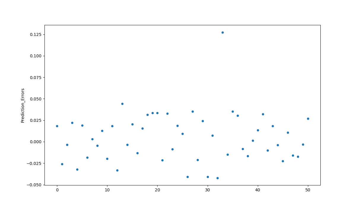
Calculate the mean-squared errors.
regression_errors.std()
Prediction_Errors    0.018801
dtype: float64
3. Pytorch
Pytorch is a machine learning and deep neural network framework from Facebook research. It is similar to the numpy framework, but with GPU acceleration. Pytorch is more flexible compared to Tensorflow (below), but usually requires more code.
import torch
import torch.nn as nn
import torch.nn.functional as F
from torch.utils.data import DataLoader
batch_size = 5
train_dl = DataLoader(train, batch_size, shuffle=False)

spy_torch = torch.Tensor([[x] for x in list(train.spy)])
target_torch = torch.Tensor([[x] for x in list(train.target)])
The index model regression is simple, and so we'll create a similarly simply neural network below by subclassing the torch.nn.Module.
# define a network
class Net(torch.nn.Module):
    def __init__(self, n_feature, n_hidden, n_output):
        super(Net, self).__init__()
        self.hidden = torch.nn.Linear(n_feature, n_hidden)
        self.predict = torch.nn.Linear(n_hidden, n_output)

    def forward(self, x):
        x = F.relu(self.hidden(x))
        x = self.predict(x)
        return x

net = Net(n_feature=1, n_hidden=100, n_output=1)
optimizer = torch.optim.SGD(net.parameters(), lr=0.2)
loss_func = torch.nn.MSELoss()  # mean squared error loss
# train the network
x = spy_torch
y = target_torch

for t in range(500):

    prediction = net(x)     # input the market returns and predict

    loss = loss_func(prediction, y)

    optimizer.zero_grad()   # zero out gradients
    loss.backward()         # backprop, compute gradients
    optimizer.step()
## Prediction Errors
spy_test_torch = torch.Tensor([[x] for x in list(test.spy)])
target_test_torch = torch.Tensor([[x] for x in list(test.target)])

preds_torch = net(spy_test_torch)
error_torch = preds_torch - target_test_torch
Calculate mean-squared error.
error_torch.std()
tensor(0.0254, grad_fn=<StdBackward0>)
And the results are slightly worse.
4. Keras/Tensorflow
import tensorflow as tf

from tensorflow import keras
from tensorflow.keras import layers
from tensorflow.keras.layers.experimental import preprocessing
index_model = tf.keras.Sequential([
    layers.Dense(units=1)
])
index_model.compile(
    optimizer=tf.optimizers.Adam(learning_rate=0.1),
    loss='mean_absolute_error')
None
history = index_model.fit(
    train.spy, train.target,
    epochs=100,
    verbose=0,
    # Calculate validation results on some percent of the training data
    validation_split = 0.2)
test_results = {}

test_results['index_model'] = index_model.evaluate(
    test.spy,
    test.target, verbose=0)
Calculate predictions in the test data set.
tensorflow_predictions = index_model.predict(test.spy)
error_tensorflow = tensorflow_predictions - test.target.values
error_tensorflow.std()
0.03595855441787083
Which is slightly more than the mean-squared error for the Pytorch network.
5. Conclusion
Arguably, we could improve these neural networks and lower their prediction errors (feel free to do this as a bonus exercise). That said, it seems that a simple linear equation (as in the regression) explains the relationship between the stock and market returns well. Remember, deep neural networks are powerful because they can approximate any arbitrary (unknown) functional relationship. But if we know the appropriate relationship, then neural nets lose their edge.